Plot electrode positions

We need to import some functions.

from eeg_positions import get_elec_coords, plot_coords

Let’s start with the basic 10-20 system in two dimensions:

coords = get_elec_coords(
    system="1020",
    dim="2d",
)

This function returns a pandas.DataFrame object:

coords.head()

	label	x	y
0	Cz	0.0	0.000000
1	Fpz	0.0	0.726585
2	Fz	0.0	0.324931
3	Pz	0.0	-0.324931
4	Oz	0.0	-0.726585

Now let’s plot these coordinates. We can supply some style arguments to eeg_positions.plot_coords() to control the color of the electrodes and the text annotations.

fig, ax = plot_coords(
    coords, scatter_kwargs={"color": "g"}, text_kwargs={"fontsize": 10}
)

fig

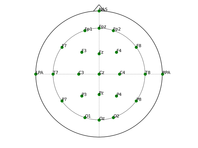
<Figure size 640x480 with 1 Axes>

Notice that the “landmarks” NAS, LPA, and RPA are included. We can drop these by passing drop_landmarks=True to get_elec_coords():

coords = get_elec_coords(
    system="1020",
    drop_landmarks=True,
    dim="2d",
)

fig, ax = plot_coords(
    coords, scatter_kwargs={"color": "g"}, text_kwargs={"fontsize": 10}
)

fig

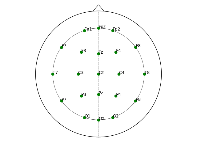
<Figure size 640x480 with 1 Axes>

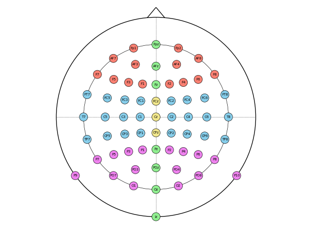
Often, we might have a list of electrode names that we would like to plot. For example, let’s assume we have the following 64 channel labels (based on the 10-05 system):

chans = """Fp1 AF7 AF3 F1 F3 F5 F7 Fp2 AF8 AF4 F2 F4 F6 F8 FT7 FC5 FC3
FC1 C1 C3 C5 T7 TP7 CP5 CP3 CP1 FT8 FC6 FC4 FC2 C2 C4 C6 T8 TP8 CP6 CP4
CP2 P1 P3 P5 P7 P9 PO7 PO3 O1 P2 P4 P6 P8 P10 PO8 PO4 O2 Iz Oz POz Pz
Fz AFz Fpz CPz Cz FCz""".split()

Many experiments aggregate electrodes into regions of interest (ROIs), which we could visualize with different colors. Let’s get their coordinates first:

coords = get_elec_coords(elec_names=chans)

Now we specifiy individual colors using the scatter_kwargs` argument. We create a list of 64 colors corresponding to our 64 coordinates (in the original order as provided by chans):

colors = (
    ["salmon"] * 14
    + ["skyblue"] * 24
    + ["violet"] * 16
    + ["lightgreen"] * 7
    + ["khaki"] * 3
)

fig, ax = plot_coords(
    coords,
    scatter_kwargs={
        "s": 150,  # electrode size
        "color": colors,
        "edgecolors": "black",  # black electrode outline
        "linewidths": 0.5,  # thin outline
    },
    text_kwargs={
        "ha": "center",  # center electrode label horizontally
        "va": "center",  # center electrode label vertically
        "fontsize": 5,  # smaller font size
    },
)

We can also plot in 3D. Let’s pick a system with more electrodes now:

coords = get_elec_coords(
    system="1010",
    drop_landmarks=True,
    dim="3d",
)

fig, ax = plot_coords(coords, text_kwargs=dict(fontsize=7))

fig

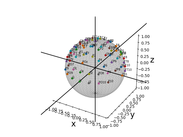
<Figure size 640x480 with 1 Axes>

When using these commands from an interactive Python session, try to set the IPython magic %matplotlib or %matplotlib qt, which will allow you to freely view the 3D plot and rotate the camera.